Monopsony II — fine-tuned text embeddings as DML controls
Part 2 of a three-post series. Part 1 estimated the partially linear coefficient with hand-coded controls only. This post appends the fine-tuned DeBERTa embedding of each HIT’s title and description.
The model is exactly the same as in Monopsony I:
\[\log(\text{duration}_i) \;=\; \theta_0 \cdot \log(\text{reward}_i) \;+\; g_0(X_i) \;+\; \varepsilon_i, \qquad E[\varepsilon_i \mid X_i, D_i] = 0.\]Only $X_i$ changes. We augment the hand-engineered controls with embeddings, retrieved from a DeBERTa-v3 language model that we fine-tune to our setting.
In this part, we discuss two things: First, we explain what embeddings are, how fine-tuning works, and we describe our specific implementation choices. Second, we explain how the fine-tuning process is integrated into the DML framework.
Embeddings and fine-tuning
Embeddings and choice of language model
Embeddings are fixed-length vector representations of strings, retrieved from a language model such as a transformer. The appeal of using embeddings over hand-engineered features is that they can capture concepts that might be overlooked by manual coding. For example, the tasks “transcribe 20 audio clips” versus “label sentiment in 100 tweets” differ in cognitive load, reading time, and recruiter requirements in ways that ad-hoc engineered features may fail to capture.
We specifically use the [CLS] token from DeBERTa-v3-base, which gives us a 768-dimensional vector. We opt here for DeBERTa-v3-base because it is a small bi-directional encoder model that allows us to retrieve embeddings at low cost and fine-tune it to our specific context. “Bi-directional” here means that the [CLS] token accommodates dependencies across the entire string sequence, not just a one-directional link from previous to subsequent tokens.
Larger reasoning models such as Qwen3 or Gemini are possible alternatives. They benefit from substantially more pretraining data and tend to produce better representations when there is limited training data and on tasks requiring nuanced reasoning. However, even the smallest Qwen3 embedding variant has roughly an order of magnitude more parameters than DeBERTa-v3-base, making both fine-tuning and inference markedly more expensive. In our setting, as we explain below, we need to repeat the fine-tuning process for each fold and outcome, which is why a smaller model such as DeBERTa-v3-base is attractive.
How to fine-tune
A pretrained language model is trained on a generic corpus with a general objective. Fine-tuning adapts the model parameters using contextual data. The language model acts as a backbone on which a small regression head is placed. In our context, we use log reward and log duration as separate outcomes and link these to the text via a tokenizer (which converts strings to indices), a backbone language model (DeBERTa) and a regression head (linear regression). After fine-tuning, the regression head is discarded and only the embeddings are retrieved, which are used as inputs for a downstream machine learner.
LoRA, not full fine-tuning
Full fine-tuning would update all 184M DeBERTa parameters. To limit the computational complexity, we use Low-Rank Adaptation (Hu et al., 2021) instead of full fine-tuning. LoRA freezes the pretrained weight matrices $W$ and inserts trainable rank-$r$ updates $\Delta W$ into the attention projections:
\[W_{\text{adapted}} \;=\; W_{\text{frozen}} \;+\; \Delta \underbrace{W}_{\text{trainable, rank } r}\]As a consequence, the LoRA fine-tuning process is much faster, while often yielding similar prediction performance compared to full fine-tuning.
Fine-tuning implementation details
A few implementation details: The text input is the concatenation of HIT title and description, tokenized by DeBERTa’s own SentencePiece tokenizer and truncated to 160 tokens. We train with the AdamW optimizer at learning rate $2 \times 10^{-4}$ (LoRA needs a higher LR than full fine-tuning because only the low-rank factors move), batch size 32, for three epochs.
Integrating fine-tuning into DML
How do we integrate fine-tuning into the DML algorithm? A naive approach might proceed as follows: using the full sample, fine-tune DeBERTa separately on log reward and log duration, retrieve the fine-tuned embeddings, and use these as inputs along with hand-coded controls in the cross-fitting process.
This approach, however, would produce predicted values that are not purely out-of-sample: we would violate the requirement that each data point not be used for both nuisance function estimation (which includes embedding estimation) and structural estimation.
For the estimation process to remain leakage-free, we move the fine-tuning step inside the cross-fitting loop. The figure below walks through the procedure. We do this twice — once with $y = \log(\text{reward})$, once with $y = \log(\text{duration})$ — because each nuisance equation gets its own fine-tuned embeddings. Within each, we run a standard $K$-fold cross-fit. For every held-out fold $k$, the backbone is trained on the other $K-1$ folds only, its embeddings are concatenated with the hand-coded controls, and the downstream learner is fit on the training folds and used to predict on fold $k$.
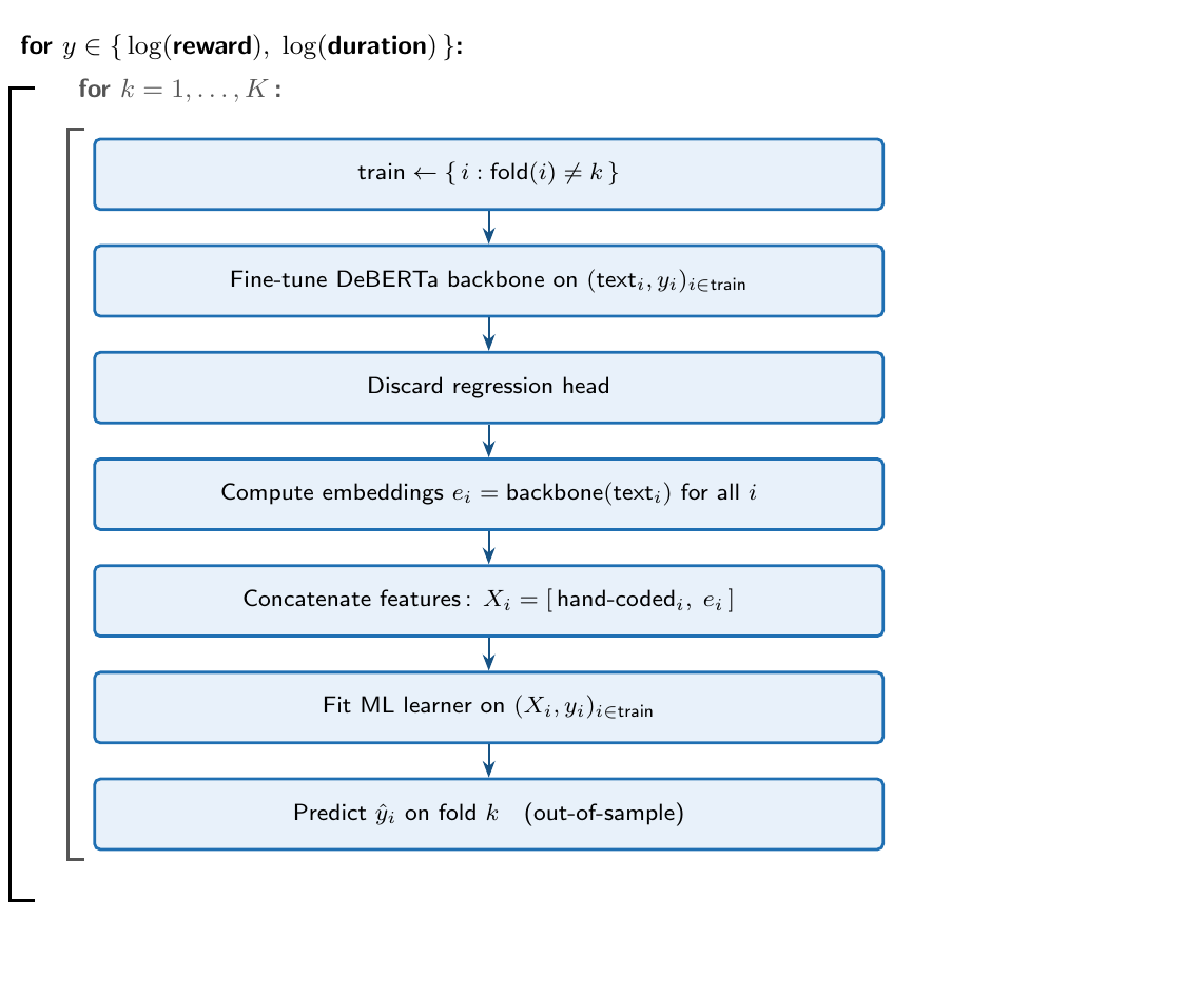
In total, we perform $2K \cdot S$ fine-tuning operations where $K=$ number of folds and $S=$ number of cross-fitting repetitions; the factor of 2 reflects the two outcomes.
Implementation of DML
Due to Python’s better LLM support, we perform the fine-tuning step in Python (saving the embeddings for each $k$ and outcome), but do the downstream nuisance function estimation and structural parameter estimation in R. The code below illustrates the implementation of cross-fitting in R for log duration and cross-fitting iteration $k$:
# retrieve fine-tuned embeddings (generated in Python & stored locally)
embed <- get_embeddings(seed = seed,k = k,
                        foldnum = K,var = "log_duration")

# column-bind hand-coded controls and embeddings
dat <- dat |> left_join(y_embed |> select(starts_with("feat_"), row_id),
                       by = c("id" = "row_id"))

# define training sample indicator
train_id <- dat$fid != k

# convert to matrix
dat <- dat |> select(log_duration, # outcome
                     time_allotted:appr_num_gt1000p, # hand-coded controls
                     starts_with("feat_") # embeddings
                     ) |>
              as.matrix()

# nuisance function estimation (here XGBoost)
fit <- mdl_xgboost( y = dat[train_id, 1],
                    X = dat[train_id, -1],
                    nrounds = 800, min_child_weight = 500,
                    eval_set = 0.1, early_stopping_rounds = 10)

# out-of-sample predicted values
hat <- predict(fit, newdata = dat[!train_id, -1])
Above, we use XGBoost as the nuisance function estimator.
The partial linear regression coefficient is then estimated using OLS (with cluster-robust standard errors):
fit_ols <- feols(resid_log_duration ~ resid_log_reward,
                  data = out,
                  cluster = ~ requester_id)
Result
Table 1: Coefficient on log(reward). Cluster-robust SE by requester_id in parentheses; cross-fitted R² reported.
| Hand-coded + fine-tuned DeBERTa embeds | |
|---|---|
| log(reward) | -0.066 (0.015) |
| n | 258352 |
| K | 3 |
| R²(Y|X) | 0.867 |
| R²(D|X) | 0.754 |
With the fine-tuned embeddings in $X$, the cross-fitted $R^2$ values are above 75% and 85%, and the cluster-robust standard error on $\hat\theta_0$ is tight enough for the point estimate to be unambiguously different from zero. $\hat\theta_0 \approx -0.066$ is in the same neighborhood as the estimate in column 9 of Table 5 (panel B) in the DML paper.
The two numbers do not coincide exactly: here we use an adapted code base and a single cross-fitting seed, and column 9 of the paper is a median-aggregated estimate over $S = 5$ seeds.
The third and final post, Monopsony III, examines robustness of the headline estimate to the seed, the choice of nuisance learner, and the construction of the cross-fitting folds.
References
- Ahrens, A., V. Chernozhukov, C. Hansen, D. Kozbur, M. Schaffer and T. Wiemann. An Introduction to Double/Debiased Machine Learning. (Working paper, this site.) §6 motivates the fine-tuned-embedding approach used here.
- Dube, A., J. Jacobs, S. Naidu and S. Suri (2020). Monopsony in online labor markets. AER: Insights 2 (1).
- He, P., J. Gao and W. Chen (2023). DeBERTa-v3.
- Hu, E. J., Y. Shen, P. Wallis, Z. Allen-Zhu, Y. Li, S. Wang, L. Wang and W. Chen (2021). LoRA: Low-Rank Adaptation of Large Language Models.
- Ahrens, A., C. B. Hansen, M. E. Schaffer and T. Wiemann (2024).
ddml: Double/debiased machine learning in R.
Continue to Monopsony III.