Monopsony I — Using DML to examine monopsony power.
This is Part 1 of a series of three posts, which revisits the Monopsony application in Section 6 of the JEL paper.
How much monopsony power does an online platform give to firms? To answer this question Dube, Jacobs, Naidu and Suri (2020) estimate the elasticity of labor supply using Amazon Mechanical Turk (MTurk).
MTurk is a marketplace for short, online tasks called HITs (Human Intelligence Tasks), e.g., labeling images, transcribing audio, filling out surveys. A recruiter posts a HIT, including a description of the task, sets a reward in dollars, and waits for workers to claim and complete it.
We discuss this application in three blog entries that complement Section 6 in our paper: Part 1 (this part) illustrates a simple DML estimation of the labor supply elasticity using only a single learner and hand-coded control variables. Part 2 incorporates unstructured text data describing the tasks using fine-tuned DeBERTa embeddings (numeric vector representations of the task text produced by DeBERTa, a pre-trained language model). Part 3 discusses validation exercises.
1. Model and identification
The estimating equation is the partially linear model considered by Dube et al. (2020):
\[\underbrace{\log(\text{duration}_i)}_{Y_i} \;=\; \theta_0 \cdot \underbrace{\log(\text{reward}_i)}_{D_i} \;+\; g_0(X_i) \;+\; \varepsilon_i, \qquad E[\varepsilon_i \mid X_i, D_i] = 0.\]where:
- $Y_i$ is the log duration it takes for HIT $i$ to be accepted;
- $D_i$ is the log reward posted by the recruiter;
- $X_i$ collects task-level controls.
The negative of $\theta_0$ is a proxy for the labor supply elasticity faced by the recruiter: If HIT are accepted more quickly when the reward rises ($\theta_0\ll 0$), labor supply is elastic. A value of $\theta_0$ close to zero — that is, when workers are unresponsive to the reward conditional on the task — indicates that recruiters have monopsony power.
MTurk tasks differ in length, complexity, qualification requirements, recruiter reputation, and content (e.g., a 30-second image label versus a 20-minute transcription). Flexibly conditioning on $X$ is thus crucial to giving $\theta_0$ a meaningful interpretation. Since tasks differ in many characteristics, this is far from trivial.
2. Data and controls
The sample is the cross-section of HITs compiled by Ipeirotis (2010), which is one of the datasets examined in Dube et al. (2020). One row is one HIT group (a batch of identical tasks posted by one recruiter).
In this post, we only consider hand-engineered controls. Fortunately, we can rely on work by Dube et al. (2020) and previous authors who have coded information on the type of tasks using the task title and descriptions. Part 2 incorporates unstructured text using fine-tuned embeddings.
The hand-coded controls fall into four blocks:
- Task design and pricing. Allotted time per HIT, the number of HITs in the batch (first/last/max), how many have already been completed at observation, the recruiter’s rate of completed HITs, indicators for time mentioned in the title/keywords.
- Qualifications and access. Indicators for whether the recruiter requires a qualification (and how long that requirement is), the number of distinct qualifications required, approval-rate and approval-count thresholds, and a custom-qualification flag.
- Recruiter aggregates. Log average reward and log average duration across all of the recruiter’s other HITs.
- Task content. Binary bag-of-words indicators for keywords/title/description tokens, plus task-category dummies (image labeling, transcription, survey, etc.) — these are the ad-hoc representation of the task text that Part 2 will replace with DeBERTa embeddings.
We perform minimal data processing: continuous variables are log(1+x) transformed and top-1% winsorized if they are right-skewed; other variables with concentrated distributions are dichotomized or discretized into a small set of indicators.
3. Estimation
We start with a simple nuisance learner: linear lasso, implemented using the ddml package with mdl_glmnet and a cross-validated penalty parameter.
We use $K = 3$ cross-fitting folds, constructed at the recruiter level — i.e., all HITs from the same requester_id are kept in the same fold. This way we respect the dependence structure of the data and are consistent with the use of cluster-robust standard errors. The figure below sketches the DML procedure.
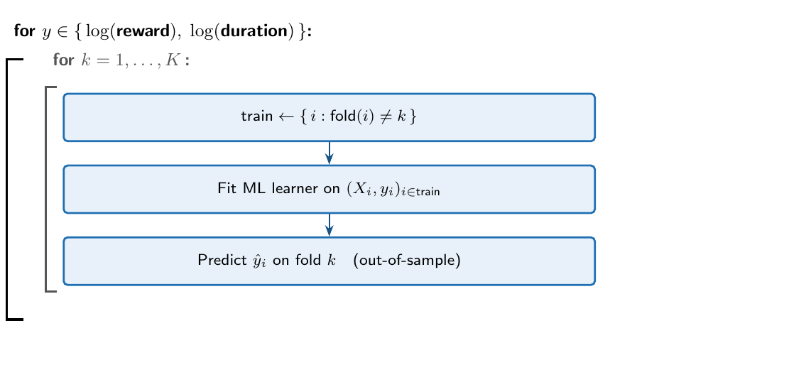
We can use the ddml package so that we don’t have to implement the DML algorithm manually. We use the ddml_plm command (where plm is short-hand for partially linear model).
set.seed(42)

lasso_spec <- list(
  what = mdl_glmnet,
  args = list(alpha = 1)
)

fit <- ddml_plm(
  y = y, D = D, X = X, # X = hand-coded controls only
  learners         = lasso_spec,
  sample_folds     = 3,
  cluster_variable = dat$requester_id
)
summary(fit)
A note on usage of ddml: passing the cluster_variable option does two things at once. It tells ddml_plm to keep each recruiter’s HITs together when constructing folds (so that no recruiter is “leaked” across the train/predict split), and it switches the standard error to cluster-robust on the same variable.
4. Result
Table 1: Coefficient on log(reward). Cluster-robust SE by requester_id in parentheses.
| DML | |
|---|---|
| log(reward) | 0.024 (0.523) |
| n | 258352 |
| K | 3 |
| R²(Y|X) | 0.687 |
| R²(D|X) | 0.743 |
Our first DML estimate is $0.024$ (with a standard error of $0.523$), indicating that $\theta_0$ is very imprecisely estimated. The cross-fitted $R^2$ values tell us how predictable the outcome and the treatment are using the hand-coded controls. With CV-lasso on the hand-coded block alone, $R^2(Y \mid X)$ sits in the high-60s and $R^2(D \mid X)$ at around 74%.
5. Next steps
We shouldn’t take this estimate very seriously: First, we haven’t validated the use of lasso against other nuisance function estimators. Second, the hand-coded variables might still miss out on important patterns in the data that are not captured through ad-hoc manual coding.
For these reasons, in the next post we will leverage fine-tuned DeBERTa embeddings to better approximate task types. The third post will refine the DML model and perform validation checks.
6. References
- Ahrens, A., V. Chernozhukov, C. Hansen, D. Kozbur, M. Schaffer and T. Wiemann. An Introduction to Double/Debiased Machine Learning. (Working paper, this site.)
- Ahrens, A., C. B. Hansen, M. E. Schaffer, and T. Wiemann (2024).
ddml: Double/Debiased machine learning in R. - Chernozhukov, V., D. Chetverikov, M. Demirer, E. Duflo, C. Hansen, W. Newey, and J. Robins (2018). Double/Debiased machine learning for treatment and structural parameters.
- Dube, A., J. Jacobs, S. Naidu and S. Suri (2020). Monopsony in online labor markets. AER: Insights 2 (1).
- Ipeirotis, P. G. (2010). Analyzing the Amazon Mechanical Turk marketplace.
Continue: Monopsony II · Monopsony III.