Dynamic Effects on Hospitalization
Setting
We follow Dobkin et al. (2018) in estimating the causal effect of hospital admissions on out-of-pocket medical spendings.1 This application is instructive in that it illustrates how DML can be used for difference-in-difference analyses. The analysis of Dobkin et al. (2018) was reconsidered by Sun & Abraham (2021) to illustrate their proposed DiD estimator.
The demonstration here is a simplified version of the analysis presented in Section 5 of our review paper. For the full replication code, see our replication repository (Link to be added).
The variables used are:
| Variable | Description |
|---|---|
oop_spend | Out of pocket medical expenditures prev 12 months |
first_hosp | First hospitalization |
hhidpn | Household/person indicator |
wave | Wave indicator |
ragey_b | Age in years |
female | Female indicator |
black | Black indicator |
hispanic | Hispanic indicator |
race_other | Other race |
hs_grad | High school graduate |
some_college | College degree |
collegeplus | Higher than college education |
Data and model set-up
We begin by loading the data, and specifying settings for a number of nuisance function estimators that we will use below. We consider OLS/logit as parametric reference specifications, (logistic) lasso and ridge, and three random forest learners.
R code
Note that for the DiD analyses to run in R, you will need to install a modified version of the original did package by Callaway & Santa’Anna.
# Hard-coded hyperparameters
library("did")
#devtools::install_github("thomaswiemann/did",ref="dev-ddml")
library(ddml)
library(readr)

dat <- read_csv("https://dmlguide.github.io/assets/dta/HRS_long.csv")

# Learners for E[Y|D=0,X] estimation
learners = list(
  list(fun = ols),
  list(fun = mdl_glmnet,
      args = list(alpha = 1)),
  list(fun = mdl_glmnet,
       args = list(alpha = 0)),
  list(fun = mdl_ranger,
      args = list(num.trees = 1000, # random forest, high regularization
                  min.node.size = 100)),
  list(fun = mdl_ranger,
      args = list(num.trees = 1000, # random forest, medium regularization
                  min.node.size = 10)),
  list(fun = mdl_ranger,
      args = list(num.trees = 1000, # random forest, low regularization
                  min.node.size = 1)))

# Hard-code learners for treatment reduced-form
learners_DX = list(
  list(fun = mdl_glm,
      args = list(family = "binomial")),
  list(fun = mdl_glmnet,
      args = list(family = "binomial", # logit-lasso
                  alpha = 1)),
  list(fun = mdl_glmnet,
      args = list(family = "binomial", # logit-ridge
                  alpha = 0)),
  list(fun = mdl_ranger,
      args = list(num.trees = 1000, # random forest, high regularization
                  min.node.size = 100)),
  list(fun = mdl_ranger,
      args = list(num.trees = 1000, # random forest, medium regularization
                  min.node.size = 10)),
  list(fun = mdl_ranger,
      args = list(num.trees = 1000, # random forest, low regularization
                  min.node.size = 1)))
DiD estimation with parametric nuisance functions
For comparison, we employ the Callway & Sant’Anna estimator of group-time average treatment effects (GT-ATT). Each GT-ATT corresponds to the ATT of a hospitalization occuring at time $g$ on out-of-pocket medical spending at time $t$. We also consider the Sant’Anna & Zhao (2020) estimator that adjust for covariates using a doubly robust scores. Unlike DML, their estimator does not employ sample-splitting and assumes that the nuisance functions follow a parameteric form.
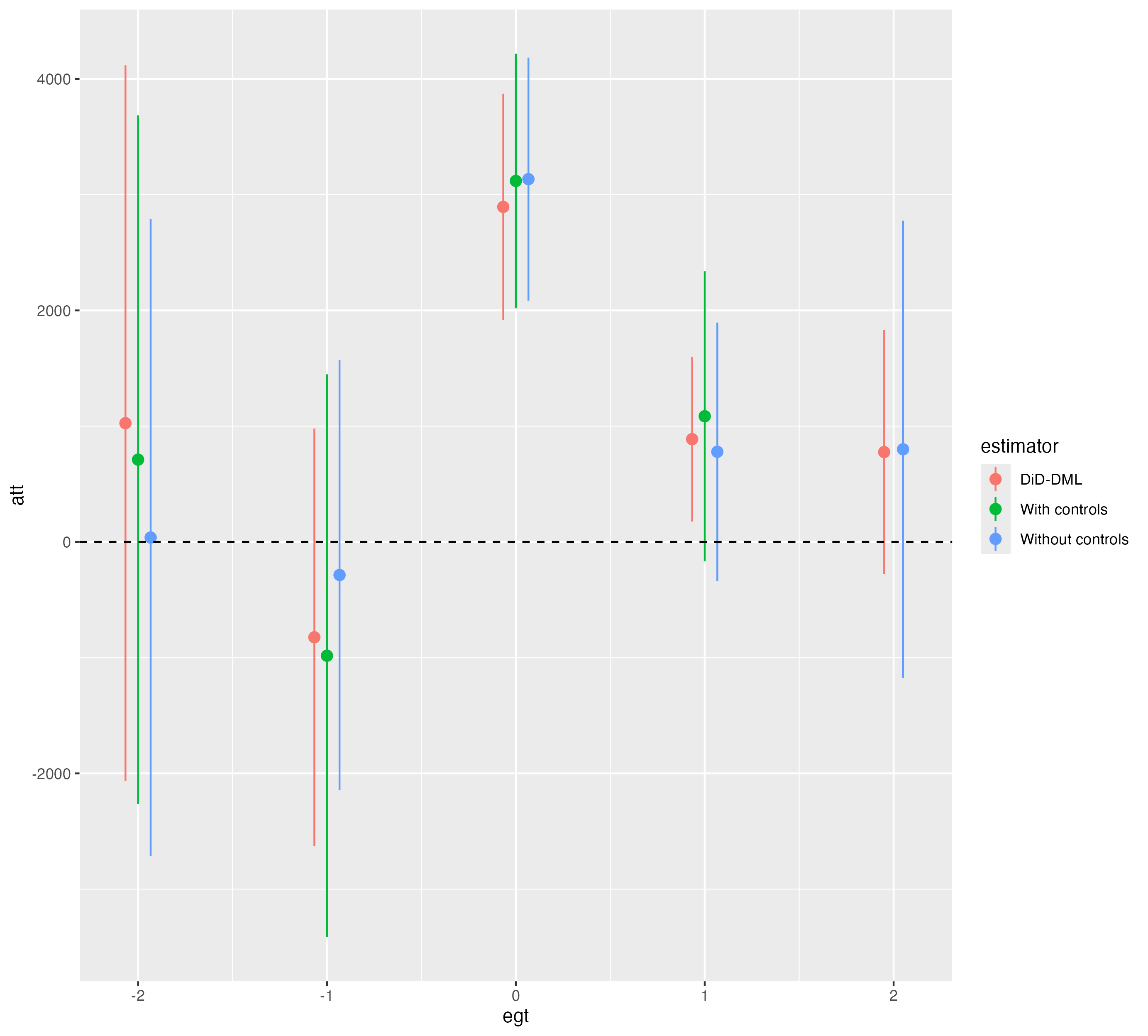
The GT-ATT estimates are then aggregated to obtain dynamic effects for up to two periods before and after the treatment onsets.
R code
# Without controls
attgt_0 <- att_gt(yname = "oop_spend",
                  gname = "first_hosp",
                  idname = "hhidpn",
                  tname = "wave",
                  control_group = "notyettreated",
                  xformla = NULL,
                  data = dat,
                  bstrap=FALSE)
# Aggregation
dyn_0 <- aggte(attgt_0, type = "dynamic", bstrap = FALSE)

# With controls
attgt_lm <- att_gt(yname = "oop_spend",
                   gname = "first_hosp",
                   idname = "hhidpn",
                   tname = "wave",
                   control_group = "notyettreated",
                   xformla = ~ ragey_b+ragey_b^2+ragey_b^3+female+black+
                     hispanic+race_other+hs_grad+some_college+collegeplus,
                   data = dat,
                   bstrap=FALSE,
                   est_method = "dr",
                   learners = list(list(fun = ols)),
                   learners_DX = list(list(fun = mdl_glm,
                                           args = list(family = binomial))),
                   type = "average",
                   trim = 0.001)
# Aggregation
dyn_lm <- aggte(attgt_lm, type = "dynamic", bstrap = FALSE)
R output
> attgt_0

Call:
att_gt(yname = "oop_spend", tname = "wave", idname = "hhidpn",
    gname = "first_hosp", xformla = NULL, data = dat, control_group = "notyettreated",
    bstrap = FALSE)

Reference: Callaway, Brantly and Pedro H.C. Sant'Anna.  "Difference-in-Differences with Multiple Time Periods." Journal of Econometrics, Vol. 225, No. 2, pp. 200-230, 2021. <https://doi.org/10.1016/j.jeconom.2020.12.001>, <https://arxiv.org/abs/1803.09015>

Group-Time Average Treatment Effects:
 Group Time  ATT(g,t) Std. Error [95% Pointwise  Conf. Band]
     8    8 3028.6250   913.4765       1238.2440    4819.006 *
     8    9 1247.6922   860.7461       -439.3392    2934.724
     8   10  800.1065  1007.5356      -1174.6271    2774.840
     9    8 -169.9604  1128.4012      -2381.5861    2041.665
     9    9 3324.3702   958.7806       1445.1947    5203.546 *
     9   10  106.8378   650.6511      -1168.4149    1382.091
    10    8   37.8749  1403.3889      -2712.7167    2788.467
    10    9 -410.5810  1027.0575      -2423.5767    1602.415
    10   10 3091.5084   995.4291       1140.5031    5042.514 *
---
Signif. codes: `*' confidence band does not cover 0

P-value for pre-test of parallel trends assumption:  0.94949
Control Group:  Not Yet Treated,  Anticipation Periods:  0
Estimation Method:  Doubly Robust
Stata code (to be added)
To be added.
Stata output (to be added)
To be added.
Double Machine Learning DiD estimation
We move to the DML estimation. The code uses the same doubly robust (and Neyman-orthogonal) score as Sant’Anna & Zhao (2020) to estimate the GT-ATT effects. However, DML uses cross-fitting which (in combination with the Neyman-orthogonal score) allows us to leverage nonparametric learners.
R code
attgt_dml <- att_gt(yname = "oop_spend",
                    gname = "first_hosp",
                    idname = "hhidpn",
                    tname = "wave",
                    control_group = "notyettreated",
                    xformla = ~ ragey_b+female+black+
                      hispanic+race_other+hs_grad+some_college+collegeplus,
                    data = dat,
                    bstrap=FALSE,
                    est_method = "ddml",
                    learners=learners,
                    learners_DX=learners_DX,
                    ensemble_type="nnls",
                    sample_folds=15,
                    shortstack=TRUE,
                    trim = 0.001,
                    silent=FALSE)
dyn_dml <- aggte(attgt_dml, type = "dynamic", bstrap = FALSE)
Stata code (to be added)
To be added.
Results
Finally, we prepare a plot to display the results:
R results
res <- bind_rows(
  data.frame(egt=dyn_dml$egt,att=dyn_dml$att.egt,se=dyn_dml$se.egt,estimator="DiD-DML"),
  data.frame(egt=dyn_lm$egt,att=dyn_lm$att.egt,se=dyn_lm$se.egt,estimator="With controls"),
  data.frame(egt=dyn_0$egt,att=dyn_0$att.egt,se=dyn_0$se.egt,estimator="Without controls")
)
res |>
  ggplot() +
  geom_pointrange(aes(x=egt,y=att,
                      ymin=att-1.96*se,ymax=att+1.96*se,
                      color=estimator),position=position_dodge(width=0.2)) +
  geom_hline(yintercept=0,linetype="dashed")

Stata results (to be added)
To be added.
-
The full data is available from the OpenICPSR repository. We consider here the subset of the data that that was also considered by Sun & Abraham (2021). ↩